The Riddler- Baseball Division Champs

\[ \newcommand{\pmi}{\operatorname{pmi}} \newcommand{\inner}[2]{\langle{#1}, {#2}\rangle} \newcommand{\Pb}{\operatorname{Pr}} \newcommand{\E}{\mathbb{E}} \newcommand{\RR}{\mathbf{R}} \newcommand{\script}[1]{\mathcal{#1}} \newcommand{\argmin}[2]{\underset{#1}{\operatorname{argmin}} {#2}} \newcommand{\optmin}[3]{ \begin{align*} & \underset{#1}{\text{minimize}} & & #2 \\ & \text{subject to} & & #3 \end{align*} } \newcommand{\optmax}[3]{ \begin{align*} & \underset{#1}{\text{maximize}} & & #2 \\ & \text{subject to} & & #3 \end{align*} } \newcommand{\optfind}[2]{ \begin{align*} & {\text{find}} & & #1 \\ & \text{subject to} & & #2 \end{align*} } \]

The Riddler column on FiveThirtyEight this week seemed like a straight forward probability problem:

Assume you have a sport (let’s call it “baseball”) in which each team plays 162 games in a season. Assume you have a division of five teams (call it the “AL East”) where each team is of exact equal ability. Specifically, each team has a 50 percent chance of winning each game. What is the expected value of the number of wins for the team that finishes in first place?

I figured the quickest way to an answer was going to be one line in Python:

>>> max((sum(random.choice((0,1)) for game in range(162)) for team in range(5)))
89

That simulates one full season and returns the number of games that the winner has won. Lets make that a function so we run the simulation many times and get the average:

def first_place_wins():
    return max((sum(random.choice((0,1)) for game in range(162)) for team in range(5)))

>>> sum(first_place_wins() for season in range(1000000))/1000000.0
88.391585

… That appears to be our answer.

After running through a million seasons, on average, the first place team will have about 88.39 wins, which is just over 7 games above .500.

Note that 1M iterations takes a few minutes as implemented, but you can get a pretty similar answer with just 50k or 100k.

A bit unsatisfying

While I trust that to be the correct answer (to some precision), it is not as satisfying as figuring out why that would be the answer. Why 7.4 games above .500 ? Does that have to do with the variance of the random variables? How can we arrive at that answer without a simulation?

First thoughts

In my first glance at the problem, it was clear that each team has the same expected number of wins in a season, 81, from just doing \(0.5 \times 162\). However, because there are five of these teams all acting independently (the problem didn’t say anything about the teams only playing each other) each with some variance, you certainly wouldn’t expect the highest team to only have 81 wins. It has to be higher than that.

Distilling the problem

The tricky part about this problem is the max that is involved in it. We can translate ...the team that finishes in first place to the max of the five teams. This means we are finding the expected value of the max of five random variables.

The five teams are acting as binomial random variables with \(p = 0.5, n = 162\).

If each team is a random variable \(T_i\), we are trying to find the expected value of a new random variable, \(T_{max}\):

The PMF of each of these \(T_i\) variables is

Simplifying down

How to turn this into the PMF of \(T_{max}\)? If this were a simple pair of dice we were rolling and taxing the max, it would be easier to visualize. Picturing each die’s result on one axis, the max norm, or \(L_{\inf}\) norm, looks like a square as you move out from the center. All pairs of results along this line turn into the same max result.

Max of two dice

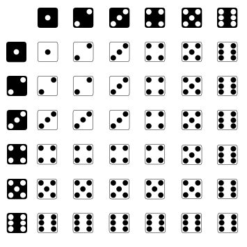
Here it’s easy to count the occurrences to enumerate the probabilities. There is one way to get a 1, three ways for a 2, five ways for a 3, etc.

Where does the formula come for this? It’s actually easier to start with the CDF of one die:

Taking the max of two dice means looking at the joint distribution. But since they are IID variables, this simplifies greatly:

This is easy to verify looking at the problem. If you picture it in terms of the box moving out, at row \(n\) of dice, there are \(n^2\) results that have a max less than or equal to \(n\).

For the PMF of each one, we would just take the CDF at \(x\) and subtract the CDF of the previous result:

This is used for the expected value:

So for the dice problem:

Tying it back

Now we just need to switch two dice rolling (uniform distributions) for 5 teams playing games (binomial distributions). The idea of raising the CDFs to the power of the number of attempts still holds, though the CDFs will be different.

Luckily, Python makes it easier to calculate a binomial distribution CDF with scipy. Below, binom_dist is an example of scipy.stats.binom.

We first make a function to get the PDF of \(T_{max}\):

def pdf_max(binom_dist, x, n):
    '''Calculates a probability value at x from the PDF of a random variable
    equal to the max of n IID binomial distributions, binom_dist'''
    return (binom_dist.cdf(x) ** n ) - (binom_dist.cdf(x-1) ** n)

Then we create the binomial distribution for the season.

binom_dist = scipy.stats.binom(162, 0.5)

The final part is the expected value:

>>> sum(pdf_max(binom_dist, i) * i for i in range(1,163))
88.394307711000806

It matches! hurray!

Code extras

To make the original a gross one-liner:

from random import random
sum(
    max((sum(random() < 0.5 for game in range(162)) for team in range(5))) 
    for season in range(100000)
)/100000.0